Fitting and simulating travel probability
Source:vignettes/V4_fitting_prob_travel.Rmd
V4_fitting_prob_travel.RmdBuild data vectors
The travel probability model requires two pieces of information: the number of trips for the time interval that travel outside the origin location (\(y_i\)) and the total number of trips observed for that origin (\(m_i\)). Both vectors must be the same length but they can have missing values (NA) that represent an unobserved origin location. The get_stay_data() function can be used to build trips for each location that are aggregated to a desired spatial scale (e.g. admin level 1 or admin level 2).
stay_data <- get_stay_data(travel_data_sim, agg_adm=2)
#> Added missing unique location names.
#> Using total trip count method
y <- setNames(stay_data$travel, stay_data$orig_id)
m <- setNames(stay_data$total, stay_data$orig_id)

n_orig <- length(y)
miss <- sample(1:n_orig, n_orig*0.2) # missing observations
y[miss] <- m[miss] <- NA

y
#> A_B_C A_B_D A_B_E A_B_G A_B_H A_B_I A_B_J A_B_K A_B_N A_B_O A_B_Q A_B_R A_B_S
#>    21   176   904     5     0    NA   331   250    74    NA    36    23   346
#> A_B_T A_B_V A_B_Y A_B_Z
#>     6    44    NA    26
m
#> A_B_C A_B_D A_B_E A_B_G A_B_H A_B_I A_B_J A_B_K A_B_N A_B_O A_B_Q A_B_R A_B_S
#>  1150   384  1941   531   322    NA   896  1421   577    NA  1593  1217   703
#> A_B_T A_B_V A_B_Y A_B_Z
#>  1035  1254    NA  1218
Estimate probability of travel for each location
To estimate the probability of traveling outside the origin location \(i\), the fit_prob_travel() function uses a Beta-Binomial model with hierarchical structure to infer travel probability in unobserved locations. \[
y_i \sim \text{Binom}(\tau_i, \sum_{\forall j} m_{ij})
\] The random variable \(y_i\) is the observed number of trips that leave origin \(i\) within the time interval. Binomial parameters \(\tau_i\) and \(\sum_{\forall j} m_{ij}\) are the success probability and total number of observed trips emanating from origin \(i\) respectively. \[
\begin{aligned}
\tau_i &\sim \text{Beta}(1+\alpha, 1+\beta) \\
\tau_\text{pop} &\sim \text{Beta}(1+\bar{\alpha}, 1+\bar{\beta})
\end{aligned}
\] Binomial probabilities for each origin \(\tau_i\) are drawn from a Beta distributed prior with shape and rate parameters \(\alpha\) and \(\beta\). The hierarchical structure comes from estimating \(\alpha\) and \(\beta\) as population-level hyper-priors for the origin-level probabilities \(\tau_i\) and allowing \(\tau_\text{pop}\) to inherit the overall population-level distribution denoted as \(\bar{\alpha}\) and \(\bar{\beta}\). \[
\begin{aligned}
\alpha &\sim \text{Gamma}(0.01, 0.01) \\
\beta &\sim \text{Gamma}(0.01, 0.01)
\end{aligned}
\]
This structure allows origin locations to have probabilities \(\tau_i\) which are driven by data in each location and all unobserved locations regress to the population mean \(\tau_\text{pop}\).
prob_trav <- fit_prob_travel(travel=y, total=m)
#> These missing locations will inherit population mean:
#> A_B_I A_B_O A_B_Y
#> Compiling model graph
#>    Resolving undeclared variables
#>    Allocating nodes
#> Graph information:
#>    Observed stochastic nodes: 14
#>    Unobserved stochastic nodes: 17
#>    Total graph size: 50
#>
#> Initializing model
#>
#> NOTE: Stopping adaptation
prob_trav_smry <- summary(prob_trav, probs=c(0.025, 0.25, 0.75, 0.975))

ggplot(data=prob_trav_smry) +
  geom_point(aes(x=mean, y=names(y)), size=2) +
  ggstance::geom_linerangeh(aes(y=names(y), xmin=Q2.5, xmax=Q97.5)) +
  ggstance::geom_linerangeh(aes(y=names(y), xmin=Q25, xmax=Q75), size=1) +
  xlab('Probability of travel outside origin') + ylab('Origin') +
  xlim(0,1) +
  theme_bw() + theme(axis.text.x=element_text(size=10),
                     axis.text.y=element_text(size=10),
                     axis.title.x=element_text(size=12, margin = margin(t = 15)),
                     axis.title.y=element_text(size=12, margin = margin(r = 15)),
                     panel.border = element_rect(colour = "black", fill=NA, size=1),
                     legend.position='right')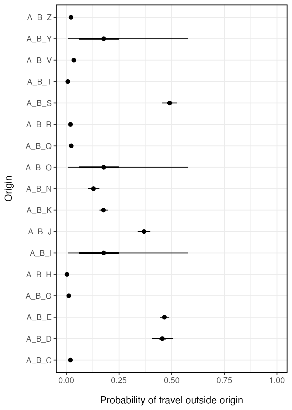
Simulate values of travel probability for each location
There can be relatively large confidence intervals around the travel probability estimated for locations without data. Since these locations inherit the population-level mean, uncertainty will likely be higher than locations with data. If we wanted to then use this model in a simulation, we may want to include this uncertainty in the model.
The predict() function can be used to simulate the fitted values of travel probability for each location. The function takes posterior estimates of the mean (\(\mu\)) and standard deviation (\(\sigma\)) for each origin \(i\), and then derives the shape and rate parameters for the Beta distribution. Simulated values are random draws from this Beta distribution.
# Simulate n realizations of travel probability for each location
predict(object=prob_trav, nsim=5, seed=123)
#>               [,1]        [,2]        [,3]        [,4]       [,5]
#> A_B_C 0.0167501135 0.018151160 0.028854062 0.019497433 0.01977168
#> A_B_D 0.5109116124 0.468652576 0.435535149 0.442645725 0.49273360
#> A_B_E 0.4701662112 0.470712361 0.466883204 0.458083855 0.47201717
#> A_B_G 0.0037315159 0.016023071 0.009027765 0.006612166 0.01022758
#> A_B_H 0.0005614135 0.000928257 0.001099007 0.000158162 0.01083817
#> A_B_I 0.1419687204 0.020947801 0.093265333 0.263929720 0.04187634
#> A_B_J 0.3845709188 0.383460726 0.380904253 0.378380234 0.36736382
#> A_B_K 0.1725927454 0.171723597 0.168009747 0.173733792 0.16084784
#> A_B_N 0.1501651371 0.111090303 0.122356879 0.121377308 0.14168614
#> A_B_O 0.1991477336 0.122187162 0.184531949 0.188267687 0.01649968
#> A_B_Q 0.0220613900 0.031613063 0.025777495 0.023579824 0.02399741
#> A_B_R 0.0213695855 0.017431353 0.018137193 0.015334299 0.01512047
#> A_B_S 0.4967676242 0.499811239 0.491572930 0.510242676 0.48024546
#> A_B_T 0.0018979450 0.010582907 0.004847146 0.004895640 0.01068822
#> A_B_V 0.0339221455 0.028713659 0.036610498 0.034745375 0.03557604
#> A_B_Y 0.0995717845 0.290348235 0.065133468 0.239565487 0.10828466
#> A_B_Z 0.0275999728 0.023907126 0.020496359 0.027937429 0.02695324
#> attr(,"model")
#> [1] "prob_travel"
#> attr(,"seed")
#> [1] 123
#> attr(,"seed")attr(,"kind")
#> attr(,"seed")attr(,"kind")[[1]]
#> [1] "Mersenne-Twister"
#>
#> attr(,"seed")attr(,"kind")[[2]]
#> [1] "Inversion"
#>
#> attr(,"seed")attr(,"kind")[[3]]
#> [1] "Rejection"